

Lesson 5: Queries and Performance Tuning
This lesson provides an overview of how Apache Cloudberry processes queries. Understanding this process can be useful when you write and tune queries.
Concepts
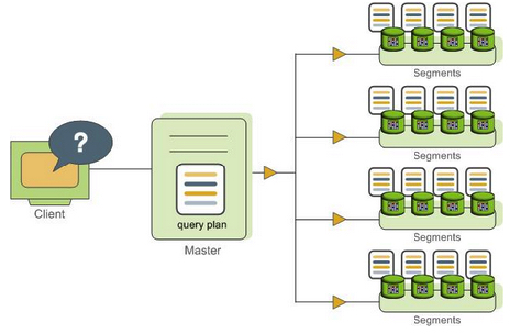
Users submit queries to Apache Cloudberry as they would to any database management system. They connect to the database instance on the Apache Cloudberry coordinator host using a client application such as psql and submit SQL statements.
Understand query planning and dispatch
The coordinator host receives, parses, and optimizes the query. The resulting query plan is either parallel or targeted. The coordinator dispatches parallel query plans to all segments, as shown in Figure 1. Each segment is responsible for executing local database operations on its own set of data query plans.
Most database operations such as table scan, join, aggregation and sort will be executed across all segments in parallel. Each operation is performed on one segment database independent of the data stored on other segment databases.
Figure 1. Dispatch the parallel query plan
Understand query plans
A query plan is a set of operations Apache Cloudberry will perform to produce the answer to a query. Each node or step in the plan represents a database operation such as a table scan, join, aggregation or sort. Plans are read and executed from bottom to top.
In addition to common database operations such as tables scan and join, Apache Cloudberry has an additional operation type called "motion". A motion operation involves moving tuples between segments during query processing.
To achieve maximum parallelism during query execution, Apache Cloudberry divides the work of a query plan into slices. A slice is a portion of the plan that segments can work on independently. A query plan is sliced wherever a motion operation occurs in the plan with one slice on each side of the motion.
Understand parallel query execution
Apache Cloudberry creates a number of database processes to handle the work of a query. On the coordinator, the query worker process is called "query dispatcher" or "QD". QD is responsible for creating and dispatching query plan. It also accumulates and presents the final results. On segments, a query worker process is called "query executor" or "QE". QE is responsible for completing its portion of work and communicating its intermediate results to other worker processes.
There is at least one worker process assigned to each slice of the query plan. A worker process works on its assigned portion of the query plan independently. During query execution, each segment will have a number of processes working on the query in parallel.
Related processes that are working on the same slice of the query plan but on different segments are called "gangs". As a portion of work is completed, tuples flow up the query plan from one gang of processes to the next. This inter-process communication between segments is referred to as the interconnect component of Apache Cloudberry.
The following section introduces some of the basic principles of query and performance tuning in a Apache Cloudberry.
Some items to consider in performance tuning:
- VACUUM and ANALYZE
- Explain plans
- Indexing
- Column or row orientation
- Set based vs. row based
- Distribution and partitioning
Exercises
After doing the following exercises, you are expected to finish the previous tutorial Lesson 4: Data Loading.
Analyze the tables
Apache Cloudberry uses Multi-version Concurrency Control (MVCC) to guarantee data isolation, one of the ACID properties of relational databases. MVCC allows multiple users of the database to obtain consistent results for a query, even if the data is changing as the query is being executed. There can be multiple versions of rows in the database, but a query sees a snapshot of the database at a single point in time, containing only the versions of rows that are valid at that point in time. When a row is updated or deleted and no active transactions continue to reference it, it can be removed. The VACUUM command removes older versions that are no longer needed, leaving free space that can be reused.
In a Apache Cloudberry, regular OLTP operations do not create the need for vacuuming out old rows, but loading data while tables are in use might create such a need. It is a best practice to VACUUM a table after a load. If the table is partitioned, and only a single partition is being altered, then a VACUUM on that partition might suffice.
The VACUUM FULL command behaves much differently than VACUUM, and its use is not recommended in Apache Cloudberry. It can be expensive in CPU and I/O consumption, cause bloat in indexes, and lock data for long periods of time.
The ANALYZE command generates statistics about the distribution of data in a table. In particular, it stores histograms about the values in each of the columns. The query optimizer depends on these statistics to select the best plan for executing a query. For example, the optimizer can use distribution data to decide on join orders. One of the optimizer's goals in a join is to minimize the volume of data that must be analyzed and potentially moved between segments by using the statistics to choose the smallest result set to work with first.
-
Connect to the database as
gpadminand run theANALYZEcommand on each of the tables:$ psql -U gpadmin tutorialtutorial=# ANALYZE faa.d_airports;
ANALYZE
tutorial=# ANALYZE faa.d_airlines;
ANALYZE
tutorial=# ANALYZE faa.d_wac;
ANALYZE
tutorial=# ANALYZE faa.d_cancellation_codes;
ANALYZE
tutorial=# ANALYZE faa.faa_otp_load;
ANALYZE
tutorial=# ANALYZE faa.otp_r;
ANALYZE
tutorial=# ANALYZE faa.otp_c;
ANALYZE
View EXPLAIN plans
An EXPLAIN plan explains the method the optimizer has chosen to produce a result set. Depending on the query, there can be a variety of methods to produce a result set. The optimizer calculates the cost for each method and chooses the one with the lowest cost. In large queries, cost is generally measured by the amount of I/O to be performed.
An EXPLAIN plan does not do any actual query processing work. Explain plans use statistics generated by the ANALYZE command, so plans generated before and after running ANALYZE can be quite different. This is especially true for queries with multiple joins, because the order of the joins can have a great impact on performance.
In the following exercise, you will generate some small tables that you can query and view some explain plans.
-
Enable timing so that you can see the effects of different performance tuning measures.
tutorial=# \timing on -
View the
create_sample_table.sqlscript, and then run it.tutorial=# \i create_sample_table.sqlpsql:create_sample_table.sql:1: NOTICE: table "sample" does not exist, skipping
DROP TABLE
Time: 8.996 ms
SET
Time: 0.509 ms
CREATE TABLE
Time: 20.419 ms
INSERT 0 1000000
Time: 28598.022 ms (00:28.598)
UPDATE 1000000
Time: 5176.394 ms (00:05.176)
UPDATE 50000
Time: 408.038 ms
UPDATE 1000000
Time: 3148.945 ms (00:03.149) -
Request the explain plan for the
COUNT()aggregate.tutorial=# EXPLAIN SELECT COUNT(*) FROM sample WHERE id > 100;QUERY PLAN
------------------------------------------------------------------------------------
Aggregate (cost=0.00..431.00 rows=1 width=8)
-> Gather Motion 2:1 (slice1; segments: 2) (cost=0.00..431.00 rows=1 width=1)
-> Seq Scan on sample (cost=0.00..431.00 rows=1 width=1)
Filter: (id > 100)
Optimizer: Pivotal Optimizer (GPORCA)
(5 rows)
Time: 5.635 msYou are expected to read query plans from bottom to top. In this example, there are 4 steps. First, there is a sequential scan on each segment server to access the rows. Then there is an aggregation on each segment server to produce a count of the number of rows from that segment. Then there is a gathering of the count value to a single location. Finally, the counts from each segment are aggregated to produce the final result.
The cost number on each step has a start and stop value. For the sequential scan, this begins at time zero and goes until 431.00. This is a fictional number created by the optimizer. It is not a number of seconds or I/O operations.
The cost numbers are cumulative, so the cost for the second operation includes the cost for the first operation. Notice that nearly all the time to process this query is in the sequential scan.
-
The
EXPLAIN ANALYZEcommand actually runs the query (without returning the result set). The cost numbers reflect the actual timings. It also produces some memory and I/O statistics.tutorial=# EXPLAIN ANALYZE SELECT COUNT(*) FROM sample WHERE id > 100;QUERY PLAN
----------------------------------------------------------------------------------------------------------------------------------
Finalize Aggregate (cost=0.00..463.54 rows=1 width=8) (actual time=329.600..329.602 rows=1 loops=1)
-> Gather Motion 2:1 (slice1; segments: 2) (cost=0.00..463.54 rows=1 width=8) (actual time=325.897..329.586 rows=2 loops=1)
-> Partial Aggregate (cost=0.00..463.54 rows=1 width=8) (actual time=324.713..324.716 rows=1 loops=1)
-> Seq Scan on sample (cost=0.00..463.54 rows=499954 width=1) (actual time=30.992..296.384 rows=500184 loops=1)
Filter: (id > 100)
Rows Removed by Filter: 53
Planning Time: 5.192 ms
(slice0) Executor memory: 37K bytes.
(slice1) Executor memory: 122K bytes avg x 2 workers, 122K bytes max (seg0).
Memory used: 128000kB
Optimizer: Pivotal Optimizer (GPORCA)
Execution Time: 338.004 ms
(12 rows)
Time: 343.866 ms
Change optimizers
By default, the sandbox instance disables the Pivotal Query Optimizer and you might see "legacy query optimizer" listed in the EXPLAIN output under "Optimizer status."
-
Check whether the Pivotal Query Optimizer is enabled.
$ gpconfig -s optimizerValues on all segments are consistent
GUC : optimizer
Coordinator value: on
Segment value: on -
Disable the Pivotal Query Optimizer.
$ gpconfig -c optimizer -v off --coordinatoronly20230726:14:42:31:031343 gpconfig:cdw:gpadmin-[INFO]:-completed successfully with parameters '-c optimizer -v on --coordinatoronly' -
Reload the configuration on coordinator and segment instances.
$ gpstop -u20230726:14:42:49:031465 gpstop:cdw:gpadmin-[INFO]:-Starting gpstop with args: -u
20230726:14:42:49:031465 gpstop:cdw:gpadmin-[INFO]:-Gathering information and validating the environment...
20230726:14:42:49:031465 gpstop:cdw:gpadmin-[INFO]:-Obtaining Cloudberry Coordinator catalog information
20230726:14:42:49:031465 gpstop:cdw:gpadmin-[INFO]:-Obtaining Segment details from coordinator...
20230726:14:42:49:031465 gpstop:cdw:gpadmin-[INFO]:-Cloudberry Version: 'postgres (Apache Cloudberry) 1.0.0 build dev'
20230726:14:42:49:031465 gpstop:cdw:gpadmin-[INFO]:-Signalling all postmaster processes to reload
Indexes and performance
Apache Cloudberry does not depend upon indexes to the same degree as traditional data warehouse systems. Because the segments execute table scans in parallel, each segment scanning a small part of the table, the traditional performance advantage from indexes is gone. Indexes consume large amounts of space and require considerable CPU time slot to compute during data loads. There are, however, times when indexes are useful, especially for highly selective queries. When a query looks up a single row, an index can dramatically improve performance.
In this exercise, you work with the legacy optimizer to know how index can improve performance. You first run a single row lookup on the sample table without an index, then rerun the query after creating an index.
tutorial=# SELECT * FROM sample WHERE big = 12345;

  id   |  big  | wee | stuff
-------+-------+-----+-------
 12345 | 12345 |   0 |
(1 row)

Time: 251.304 ms
tutorial=#
tutorial=# EXPLAIN SELECT * FROM sample WHERE big = 12345;

                                   QUERY PLAN
--------------------------------------------------------------------------------
 Gather Motion 2:1  (slice1; segments: 2)  (cost=0.00..8552.02 rows=1 width=15)
   ->  Seq Scan on sample  (cost=0.00..8552.00 rows=1 width=15)
         Filter: (big = 12345)
 Optimizer: Postgres query optimizer
(4 rows)

Time: 0.709 ms
tutorial=#
tutorial=#
tutorial=# CREATE INDEX sample_big_index ON sample(big);

CREATE INDEX
Time: 1574.117 ms (00:01.574)
tutorial=#
tutorial=#
tutorial=# SELECT * FROM sample WHERE big = 12345;
  id   |  big  | wee | stuff
-------+-------+-----+-------
 12345 | 12345 |   0 |
(1 row)

Time: 2.774 ms
tutorial=# EXPLAIN SELECT * FROM sample WHERE big = 12345;
                                      QUERY PLAN
--------------------------------------------------------------------------------------
 Gather Motion 2:1  (slice1; segments: 2)  (cost=0.17..8.21 rows=1 width=15)
   ->  Index Scan using sample_big_index on sample  (cost=0.17..8.19 rows=1 width=15)
         Index Cond: (big = 12345)
 Optimizer: Postgres query optimizer
(4 rows)

Time: 0.627 ms
Notice the difference in timing between the single-row SELECT with and without the index. The difference would have been much greater for a larger table, because indexes improve performance for queries on large datasets. Note that even when an index exists, the optimizer might choose not to use it if another more efficient plan is available.
View the following EXPLAIN plans to compare plans for some other common types of queries.
tutorial=# EXPLAIN SELECT * FROM sample WHERE big = 12345;
tutorial=# EXPLAIN SELECT * FROM sample WHERE big > 12345;
tutorial=# EXPLAIN SELECT * FROM sample WHERE big = 12345 OR big = 12355;
tutorial=# DROP INDEX sample_big_index;
tutorial=# EXPLAIN SELECT * FROM sample WHERE big = 12345 OR big = 12355;
Row vs. column orientation
Apache Cloudberry offers the ability to store a table in either row or column orientation. Both storage options have advantages, depending upon data compression characteristics, the kinds of queries executed, the row length, and the complexity, and the number of join columns.
As a general rule, very wide tables are better stored in row orientation, especially if there are joins on many columns. Column orientation works well to save space with compression and to reduce I/O when there is much duplicated data in columns.
In this exercise, you will create a column-oriented version of the fact table and compare it with the row-oriented version.
-
Create a column-oriented version of the FAA On Time Performance fact table and insert the data from the row-oriented version.
tutorial=# CREATE TABLE FAA.OTP_C (LIKE faa.otp_r) WITH (appendonly=true,
orientation=column)
DISTRIBUTED BY (UniqueCarrier, FlightNum) PARTITION BY RANGE(FlightDate)
( PARTITION mth START('2009-06-01'::date) END ('2010-10-31'::date)
EVERY ('1 mon'::interval));
CREATE TABLE
tutorial=#tutorial=# INSERT INTO faa.otp_c SELECT * FROM faa.otp_r;
INSERT 0 1024552 -
Compare the definitions of the row and the column versions of the table.
tutorial=# \d faa.otp_r

                Table "faa.otp_r"
       Column        |       Type       | Collation | Nullable | Default
----------------------+------------------+-----------+----------+---------
flt_year             | smallint         |           |          |
flt_quarter          | smallint         |           |          |
flt_month            | smallint         |           |          |
flt_dayofmonth       | smallint         |           |          |
flt_dayofweek        | smallint         |           |          |
flightdate           | date             |           |          |
uniquecarrier        | text             |           |          |
airlineid            | integer          |           |          |
carrier              | text             |           |          |
flightnum            | text             |           |          |
origin               | text             |           |          |
origincityname       | text             |           |          |
originstate          | text             |           |          |
originstatename      | text             |           |          |
dest                 | text             |           |          |
destcityname         | text             |           |          |
deststate            | text             |           |          |
deststatename        | text             |           |          |
crsdeptime           | text             |           |          |
deptime              | integer          |           |          |
depdelay             | double precision |           |          |
depdelayminutes      | double precision |           |          |
departuredelaygroups | smallint         |           |          |
taxiout              | smallint         |           |          |
wheelsoff            | text             |           |          |
wheelson             | text             |           |          |
taxiin               | smallint         |           |          |
crsarrtime           | text             |           |          |
arrtime              | text             |           |          |
arrdelay             | double precision |           |          |
arrdelayminutes      | double precision |           |          |
arrivaldelaygroups   | smallint         |           |          |
cancelled            | smallint         |           |          |
cancellationcode     | text             |           |          |
diverted             | smallint         |           |          |
crselapsedtime       | integer          |           |          |
actualelapsedtime    | double precision |           |          |
airtime              | double precision |           |          |
flights              | smallint         |           |          |
distance             | double precision |           |          |
distancegroup        | smallint         |           |          |
carrierdelay         | smallint         |           |          |
weatherdelay         | smallint         |           |          |
nasdelay             | smallint         |           |          |
securitydelay        | smallint         |           |          |
lateaircraftdelay    | smallint         |           |          |
Distributed by: (uniquecarrier, flightnum)
Notice that the column-oriented version is append-only and partitioned. It has seventeen child files for the partitions, one for each month from June 2009 through October 2010.
tutorial=# \d+ faa.otp_cPartitioned table "faa.otp_c"
Column | Type | Collation | Nullable | Default | Storage | Compression | Stats target | Description
----------------------+------------------+-----------+----------+---------+----------+-------------+--------------+-------------
flt_year | smallint | | | | plain | | |
flt_quarter | smallint | | | | plain | | |
flt_month | smallint | | | | plain | | |
flt_dayofmonth | smallint | | | | plain | | |
flt_dayofweek | smallint | | | | plain | | |
flightdate | date | | | | plain | | |
uniquecarrier | text | | | | extended | | |
airlineid | integer | | | | plain | | |
carrier | text | | | | extended | | |
flightnum | text | | | | extended | | |
origin | text | | | | extended | | |
origincityname | text | | | | extended | | |
originstate | text | | | | extended | | |
originstatename | text | | | | extended | | |
dest | text | | | | extended | | |
destcityname | text | | | | extended | | |
deststate | text | | | | extended | | |
deststatename | text | | | | extended | | |
crsdeptime | text | | | | extended | | |
deptime | integer | | | | plain | | |
depdelay | double precision | | | | plain | | |
depdelayminutes | double precision | | | | plain | | |
departuredelaygroups | smallint | | | | plain | | |
taxiout | smallint | | | | plain | | |
wheelsoff | text | | | | extended | | |
wheelson | text | | | | extended | | |
taxiin | smallint | | | | plain | | |
crsarrtime | text | | | | extended | | |
arrtime | text | | | | extended | | |
arrdelay | double precision | | | | plain | | |
arrdelayminutes | double precision | | | | plain | | |
arrivaldelaygroups | smallint | | | | plain | | |
cancelled | smallint | | | | plain | | |
cancellationcode | text | | | | extended | | |
diverted | smallint | | | | plain | | |
crselapsedtime | integer | | | | plain | | |
actualelapsedtime | double precision | | | | plain | | |
airtime | double precision | | | | plain | | |
flights | smallint | | | | plain | | |
distance | double precision | | | | plain | | |
distancegroup | smallint | | | | plain | | |
carrierdelay | smallint | | | | plain | | |
weatherdelay | smallint | | | | plain | | |
nasdelay | smallint | | | | plain | | |
securitydelay | smallint | | | | plain | | |
lateaircraftdelay | smallint | | | | plain | | |
Partition key: RANGE (flightdate)
Partitions: otp_c_1_prt_mth_1 FOR VALUES FROM ('2009-06-01') TO ('2009-07-01'),
otp_c_1_prt_mth_10 FOR VALUES FROM ('2010-03-01') TO ('2010-04-01'),
otp_c_1_prt_mth_11 FOR VALUES FROM ('2010-04-01') TO ('2010-05-01'),
otp_c_1_prt_mth_12 FOR VALUES FROM ('2010-05-01') TO ('2010-06-01'),
otp_c_1_prt_mth_13 FOR VALUES FROM ('2010-06-01') TO ('2010-07-01'),
otp_c_1_prt_mth_14 FOR VALUES FROM ('2010-07-01') TO ('2010-08-01'),
otp_c_1_prt_mth_15 FOR VALUES FROM ('2010-08-01') TO ('2010-09-01'),
otp_c_1_prt_mth_16 FOR VALUES FROM ('2010-09-01') TO ('2010-10-01'),
otp_c_1_prt_mth_17 FOR VALUES FROM ('2010-10-01') TO ('2010-10-31'),
otp_c_1_prt_mth_2 FOR VALUES FROM ('2009-07-01') TO ('2009-08-01'),
otp_c_1_prt_mth_3 FOR VALUES FROM ('2009-08-01') TO ('2009-09-01'),
otp_c_1_prt_mth_4 FOR VALUES FROM ('2009-09-01') TO ('2009-10-01'),
otp_c_1_prt_mth_5 FOR VALUES FROM ('2009-10-01') TO ('2009-11-01'),
otp_c_1_prt_mth_6 FOR VALUES FROM ('2009-11-01') TO ('2009-12-01'),
otp_c_1_prt_mth_7 FOR VALUES FROM ('2009-12-01') TO ('2010-01-01'),
otp_c_1_prt_mth_8 FOR VALUES FROM ('2010-01-01') TO ('2010-02-01'),
otp_c_1_prt_mth_9 FOR VALUES FROM ('2010-02-01') TO ('2010-03-01')
Distributed by: (uniquecarrier, flightnum)tutorial=# \d+ otp_c_1_prt_mth_1Table "faa.otp_c_1_prt_mth_1"
Column | Type | Collation | Nullable | Default | Storage | Compression | Stats target | Compression Type | Compression Level | Block Size | Description
----------------------+------------------+-----------+----------+---------+----------+-------------+--------------+------------------+-------------------+------------+-------------
flt_year | smallint | | | | plain | | | none | 0 | 32768 |
flt_quarter | smallint | | | | plain | | | none | 0 | 32768 |
flt_month | smallint | | | | plain | | | none | 0 | 32768 |
flt_dayofmonth | smallint | | | | plain | | | none | 0 | 32768 |
flt_dayofweek | smallint | | | | plain | | | none | 0 | 32768 |
flightdate | date | | | | plain | | | none | 0 | 32768 |
uniquecarrier | text | | | | extended | | | none | 0 | 32768 |
airlineid | integer | | | | plain | | | none | 0 | 32768 |
carrier | text | | | | extended | | | none | 0 | 32768 |
flightnum | text | | | | extended | | | none | 0 | 32768 |
origin | text | | | | extended | | | none | 0 | 32768 |
origincityname | text | | | | extended | | | none | 0 | 32768 |
originstate | text | | | | extended | | | none | 0 | 32768 |
originstatename | text | | | | extended | | | none | 0 | 32768 |
dest | text | | | | extended | | | none | 0 | 32768 |
destcityname | text | | | | extended | | | none | 0 | 32768 |
deststate | text | | | | extended | | | none | 0 | 32768 |
deststatename | text | | | | extended | | | none | 0 | 32768 |
crsdeptime | text | | | | extended | | | none | 0 | 32768 |
deptime | integer | | | | plain | | | none | 0 | 32768 |
depdelay | double precision | | | | plain | | | none | 0 | 32768 |
depdelayminutes | double precision | | | | plain | | | none | 0 | 32768 |
departuredelaygroups | smallint | | | | plain | | | none | 0 | 32768 |
taxiout | smallint | | | | plain | | | none | 0 | 32768 |
wheelsoff | text | | | | extended | | | none | 0 | 32768 |
wheelson | text | | | | extended | | | none | 0 | 32768 |
taxiin | smallint | | | | plain | | | none | 0 | 32768 |
crsarrtime | text | | | | extended | | | none | 0 | 32768 |
arrtime | text | | | | extended | | | none | 0 | 32768 |
arrdelay | double precision | | | | plain | | | none | 0 | 32768 |
arrdelayminutes | double precision | | | | plain | | | none | 0 | 32768 |
arrivaldelaygroups | smallint | | | | plain | | | none | 0 | 32768 |
cancelled | smallint | | | | plain | | | none | 0 | 32768 |
cancellationcode | text | | | | extended | | | none | 0 | 32768 |
diverted | smallint | | | | plain | | | none | 0 | 32768 |
crselapsedtime | integer | | | | plain | | | none | 0 | 32768 |
actualelapsedtime | double precision | | | | plain | | | none | 0 | 32768 |
airtime | double precision | | | | plain | | | none | 0 | 32768 |
flights | smallint | | | | plain | | | none | 0 | 32768 |
distance | double precision | | | | plain | | | none | 0 | 32768 |
distancegroup | smallint | | | | plain | | | none | 0 | 32768 |
carrierdelay | smallint | | | | plain | | | none | 0 | 32768 |
weatherdelay | smallint | | | | plain | | | none | 0 | 32768 |
nasdelay | smallint | | | | plain | | | none | 0 | 32768 |
securitydelay | smallint | | | | plain | | | none | 0 | 32768 |
lateaircraftdelay | smallint | | | | plain | | | none | 0 | 32768 |
Partition of: otp_c FOR VALUES FROM ('2009-06-01') TO ('2009-07-01')
Partition constraint: ((flightdate IS NOT NULL) AND (flightdate >= '2009-06-01'::date) AND (flightdate < '2009-07-01'::date))
Checksum: t
Distributed by: (uniquecarrier, flightnum)
Access method: ao_column -
Compare the sizes of the tables using the
pg_relation_size()andpg_total_relation_size()functions. Thepg_size_pretty()function converts the size in bytes to human-readable units.tutorial=# SELECT pg_size_pretty(pg_relation_size('faa.otp_r'));pg_size_pretty
----------------
256 MB
(1 row)tutorial=# SELECT pg_size_pretty(pg_total_relation_size('faa.otp_r'));pg_size_pretty
----------------
256 MB
(1 row)tutorial=# SELECT pg_size_pretty(sum(pg_relation_size(inhrelid))) FROM pg_inherits WHERE inhparent = 'faa.otp_c'::regclass;pg_size_pretty
----------------
403 MB
(1 row)tutorial=# SELECT pg_size_pretty(sum(pg_total_relation_size(inhrelid))) FROM pg_inherits WHERE inhparent = 'faa.otp_c'::regclass;pg_size_pretty
----------------
405 MB
(1 row)
Check for even data distribution on segments
The faa.otp_r and faa.otp_c tables use a hash distribution on the UniqueCarrier and FlightNum columns. These columns ensure an even data distribution across segments and, due to frequent joins involving them, optimize query execution by minimizing data movement between segments. When there is no benefit in co-locating data from various tables on the segments, using a unique column guarantees balanced distribution. However, using a low-cardinality column like Diverted, having only two values, results in poor distribution.
A primary goal of distribution is to have a balanced amount of data in each segment. The subsequent query demonstrates this. Given that both column-oriented and row-oriented tables share the same distribution columns, their counts should match.
tutorial=# SELECT gp_segment_id, COUNT(*) FROM faa.otp_c GROUP BY
gp_segment_id ORDER BY gp_segment_id;
 gp_segment_id | count
---------------+--------
             0 | 513746
             1 | 510806
(2 rows)
About partitioning
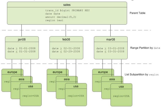
Partitioning a table can improve query performance and simplify data administration. The table is divided into smaller child files using a range or a list value, such as a date range or a country code.
Partitions can improve query performance dramatically. When a query predicate filters on the same criteria used to define partitions, the optimizer can avoid searching partitions that do not contain relevant data.
A common application for partitioning is to maintain a rolling window of data based on date, for example, a fact table containing the most recent 12 months of data. Using the ALTER TABLE statement, an existing partition can be dropped by removing its child file. This is much more efficient than scanning the entire table and removing rows with a DELETE statement.
Partitions might also be sub-partitioned. For example, a table can be partitioned by month, and the month partitions can be sub-partitioned by week. Apache Cloudberry creates child files for the months and weeks. The actual data, however, is stored in the child files created for the week subpartitions. Only child files at the leaf level hold data.
When a new partition is added, you can run ANALYZE on just the data in that partition. ANALYZE can run on the root partition (the name of the table in the CREATE TABLE statement) or on a child file created for a leaf partition. If ANALYZE has already run on the other partitions and the data is static, it is not necessary to run it again on those partitions.
Apache Cloudberry supports:
- Range partitioning: division of data based on a numerical range, such as date or price.
- List partitioning: division of data based on a list of values, such as sales territory or product line.
- A combination of both types.
The following exercise compares SELECT statements with WHERE clauses that do and do not use a partitioned column.
The column-oriented version of the fact table you created is partitioned by date. First, execute a query that filters on a non-partitioned column and note the execution time.
tutorial=# \timing on

Timing is on.

tutorial=# EXPLAIN SELECT MAX(depdelay) FROM faa.otp_c WHERE UniqueCarrier = 'UA';

NOTICE:  One or more columns in the following table(s) do not have statistics: otp_c
HINT:  For non-partitioned tables, run analyze <table_name>(<column_list>). For partitioned tables, run analyze rootpartition <table_name>(<column_list>). See log for columns missing statistics.
                                            QUERY PLAN
--------------------------------------------------------------------------------------------------
 Finalize Aggregate  (cost=0.00..531.33 rows=1 width=8)
   ->  Gather Motion 2:1  (slice1; segments: 2)  (cost=0.00..531.33 rows=1 width=8)
         ->  Partial Aggregate  (cost=0.00..531.33 rows=1 width=8)
               ->  Append  (cost=0.00..531.15 rows=204908 width=16)
                     ->  Seq Scan on otp_c_1_prt_mth_1  (cost=0.00..531.15 rows=204908 width=16)
                           Filter: (uniquecarrier = 'UA'::text)
                     ->  Seq Scan on otp_c_1_prt_mth_2  (cost=0.00..531.15 rows=204908 width=16)
                           Filter: (uniquecarrier = 'UA'::text)
                     ->  Seq Scan on otp_c_1_prt_mth_3  (cost=0.00..531.15 rows=204908 width=16)
                           Filter: (uniquecarrier = 'UA'::text)
                     ->  Seq Scan on otp_c_1_prt_mth_4  (cost=0.00..531.15 rows=204908 width=16)
                           Filter: (uniquecarrier = 'UA'::text)
                     ->  Seq Scan on otp_c_1_prt_mth_5  (cost=0.00..531.15 rows=204908 width=16)
                           Filter: (uniquecarrier = 'UA'::text)
                     ->  Seq Scan on otp_c_1_prt_mth_6  (cost=0.00..531.15 rows=204908 width=16)
                           Filter: (uniquecarrier = 'UA'::text)
                     ->  Seq Scan on otp_c_1_prt_mth_7  (cost=0.00..531.15 rows=204908 width=16)
                           Filter: (uniquecarrier = 'UA'::text)
                     ->  Seq Scan on otp_c_1_prt_mth_8  (cost=0.00..531.15 rows=204908 width=16)
                           Filter: (uniquecarrier = 'UA'::text)
                     ->  Seq Scan on otp_c_1_prt_mth_9  (cost=0.00..531.15 rows=204908 width=16)
                           Filter: (uniquecarrier = 'UA'::text)
                     ->  Seq Scan on otp_c_1_prt_mth_10  (cost=0.00..531.15 rows=204908 width=16)
                           Filter: (uniquecarrier = 'UA'::text)
                     ->  Seq Scan on otp_c_1_prt_mth_11  (cost=0.00..531.15 rows=204908 width=16)
                           Filter: (uniquecarrier = 'UA'::text)
                     ->  Seq Scan on otp_c_1_prt_mth_12  (cost=0.00..531.15 rows=204908 width=16)
                           Filter: (uniquecarrier = 'UA'::text)
                     ->  Seq Scan on otp_c_1_prt_mth_13  (cost=0.00..531.15 rows=204908 width=16)
                           Filter: (uniquecarrier = 'UA'::text)
                     ->  Seq Scan on otp_c_1_prt_mth_14  (cost=0.00..531.15 rows=204908 width=16)
                           Filter: (uniquecarrier = 'UA'::text)
                     ->  Seq Scan on otp_c_1_prt_mth_15  (cost=0.00..531.15 rows=204908 width=16)
                           Filter: (uniquecarrier = 'UA'::text)
                     ->  Seq Scan on otp_c_1_prt_mth_16  (cost=0.00..531.15 rows=204908 width=16)
                           Filter: (uniquecarrier = 'UA'::text)
                     ->  Seq Scan on otp_c_1_prt_mth_17  (cost=0.00..531.15 rows=204908 width=16)
                           Filter: (uniquecarrier = 'UA'::text)
 Optimizer: Pivotal Optimizer (GPORCA)
(39 rows)
Time: 16.113 ms
tutorial=#
tutorial=#

tutorial=# EXPLAIN SELECT MAX(depdelay) FROM faa.otp_c WHERE flightdate ='2009-11-01';

NOTICE:  One or more columns in the following table(s) do not have statistics: otp_c
HINT:  For non-partitioned tables, run analyze <table_name>(<column_list>). For partitioned tables, run analyze rootpartition <table_name>(<column_list>). See log for columns missing statistics.

                                           QUERY PLAN
------------------------------------------------------------------------------------------------
 Finalize Aggregate  (cost=0.00..470.52 rows=1 width=8)
   ->  Gather Motion 2:1  (slice1; segments: 2)  (cost=0.00..470.52 rows=1 width=8)
         ->  Partial Aggregate  (cost=0.00..470.52 rows=1 width=8)
               ->  Append  (cost=0.00..470.45 rows=81963 width=12)
                     ->  Seq Scan on otp_c_1_prt_mth_6  (cost=0.00..470.45 rows=81963 width=12)
                           Filter: (flightdate = '2009-11-01'::date)
 Optimizer: Pivotal Optimizer (GPORCA)
(7 rows)

Time: 7.434 ms
The query on the partitioned column takes much less time to execute. If you compare the explain plans for the queries in this exercise, you will see that the first query scans each of the seventeen child files, while the second scans just one child file. The reduction in I/O and CPU time explains the improved execution time.
